Subqueries and CTEs

Updated Aug 28, 2019 ·

Sample Tables

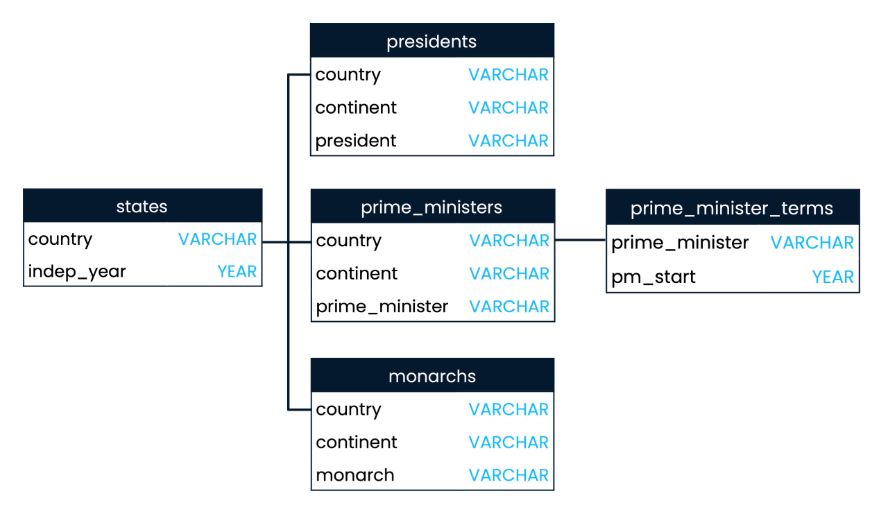
Here is the schema for the sample World table:

To download the actual files, you can get them from my Github repository.

• states.csv
• presidents.csv
• prime_ministers.csv
• prime_minister_terms.csv
• monarchs.csv

Additive Joins

In SQL, joins are typically used to combine data from two or more tables. The joins discussed in the previous pages are "additive," meaning they add columns to the original left table.

As a recap:

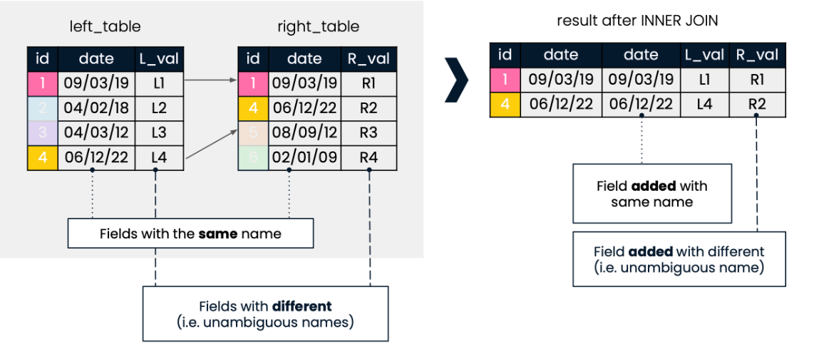
INNER JOIN adds columns to the original left table based on matching rows in both tables. For example, an INNER JOIN on the id field adds additional columns from the right table to the left table.

SELECT *
FROM left_table
INNER JOIN right_table
ON left_table.id = right_table.id;

Explanations:

• Fields with different names are added with their original names.
• Fields with the same name can result in duplicate columns, which can be renamed using aliasing.

To make it clearer, see the diagram below.

Subqueries

Subqueries are nested queries inside another query. They can simplify results and improve readability.

• Can be used in SELECT, FROM, and WHERE clauses.
• Often return single results instead of multiple rows.
• Provide a more readable alternative to complex joins.

info

Performance note: Subqueries in FROM clauses limit optimization and may reduce readability.

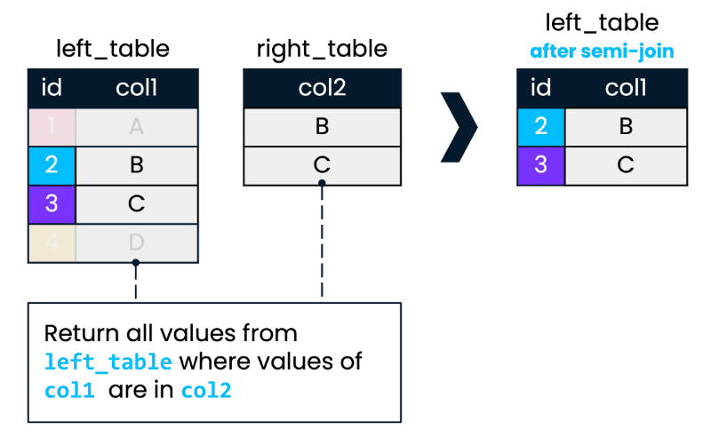
Semi Join

Semi joins differ from traditional joins in that they don't add columns from the right table. Instead, they filter the left table based on a condition in the right table. They return all rows from the left table where a specified condition is met in the right table.

Example on Semi Join

Consider the presidents and states table. Identify which countries gained independence before 1800, and then identify the presidents of those countries.

We can start with finding the countries first:

SELECT country
FROM states
WHERE indep_year < 1800; 

We can then further filter the output by using the pevious SQL statement as a subquery within another SQL statement.

SELECT country, continent, president
FROM presidents
WHERE country IN 
  (
    SELECT country
    FROM states
    WHERE indep_year < 1800
  );

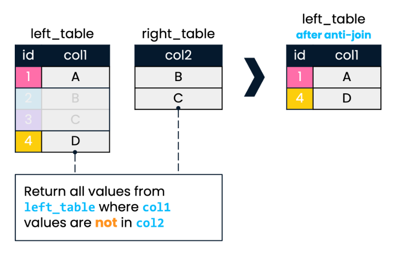
Anti Join

An anti join filters the left table by excluding rows that match a condition in the right table. It returns rows from the left table where a specified condition is NOT met in the right table.

Example of Anti Join

Consider the presidents and states table. Identify countries in the Americas founded after 1800.

SELECT country, president
FROM presidents
WHERE continent LIKE '%America'
  AND country NOT IN
  (
    SELECT country
    FROM states
    WHERE indep_year < 1800
  );

Types of Subqueries

1. SELECT Subqueries

   • Used in the SELECT clause to calculate values.
   • Avoids generating large result sets from full outer joins.
   • Example: Compare average word length in a movie script and the English language.

2. WHERE Subqueries

   • Applied in the WHERE clause to act as dynamic filters.
   • Example: Filter English words found in a movie script dynamically.

3. FROM Subqueries

   • Creates temporary result sets for the main query.
   • Better rewritten as joins for better readability and performance.

Subqueries in WHERE Clause

Subqueries are frequently used inside the WHERE clause, which allows for filtering data based on complex conditions. This is particularly useful in semi joins and anti joins.

The WHERE clause is often the go-to place for subqueries because filtering is a fundamental task in data manipulation.

Syntax for subqueries:

SELECT * 
FROM table_1 
WHERE field_1 IN
    (include subquery here)

We can then add the subquery. Note that column_name and another_column_name needs to be of the same data type for this to work. Subqueries can reference the same table or a different table, allowing for diverse query structures.

SELECT *
FROM table_name
WHERE column_name IN (
    SELECT another_column_name
    FROM another_table
    WHERE field_2 = condition
);

Subqueries in SELECT Clause

Subqueries can also be placed inside the SELECT clause to calculate or retrieve additional data that complements each row in the main query. Subqueries in the SELECT clause are often used to perform calculations or aggregations that would be cumbersome with a direct join.

info

Subqueries in SELECT and WHERE statements are analogous to JOINs

Example on Subqueries

Monarchs

Suppose we want to count the number of monarchs for each continent in a states table using data from a monarchs table. We can use a subquery to achieve this without explicitly joining the tables.

Start with the first filter, which is to get all unique continents from the prime_ministers table. This should print just the 7 continents, removing any duplicates.

SELECT DISTINCT continent
FROM prime_ministers;

Output:

continent
North America
Europe
Asia
South America
Oceania
Africa

For the next filtering, the output that we want to see should look like this:

continent	monarch_count

Let's now focus on the second column. To get the monarch_count:

SELECT COUNT(*) 
FROM monarchs 
WHERE monarchs.continent = prime_ministers.continent

Combining both SQL statements into one:

SELECT 
    DISTINCT continent,      -- this is the first SELECT statement 
    (SELECT COUNT(*)         -- this is the second SELECT statement, which is a subquery
     FROM monarchs
     WHERE monarchs.continent = prime_ministers.continent) AS monarch_count
FROM prime_ministers;

Explanation:

• This query selects distinct continents from the prime_ministers table.
• For each continent, a subquery counts the number of monarchs in the monarchs table.
• The subquery uses a WHERE clause to match the continent fields between the two tables.
• The result of the subquery is aliased as monarch_count to provide clarity in the output.

Output:

continent	monarch_count
Europe	7
North America	1
Oceania	1
Asia	1
Africa	0

Populations

Below is the populations table with 20 records inside.

populations table

pop_id	country_code	year	fertility_rate	life_expectancy	size
20	ABW	2010	1.704	74.95354	101597
19	ABW	2015	1.647	75.573586	103889
2	AFG	2010	5.746	58.97083	27962208
1	AFG	2015	4.653	60.71717	32526562
12	AGO	2010	6.416	50.65417	21219954
11	AGO	2015	5.996	52.666096	25021974
4	ALB	2010	1.663	77.03695	2913021
3	ALB	2015	1.793	78.014465	2889167
10	AND	2010	1.27	null	84419
9	AND	2015	null	null	70473
409	ARE	2010	1.868	76.67525	8329453
408	ARE	2015	1.767	77.541245	9156963
16	ARG	2010	2.37	75.48498	41222876
15	ARG	2015	2.308	76.33422	43416756
18	ARM	2010	1.648	74.22634	2963496
17	ARM	2015	1.517	74.79712	3017712
8	ASM	2010	null	null	55636
7	ASM	2015	null	null	55538
14	ATG	2010	2.13	75.30878	87233
13	ATG	2015	2.063	76.10022	91818

Goal: Figure out which countries had high average life expectancies in 2015.

Begin by calculating the average life expectancy from the populations table. Filter your answer to use records from 2015 only.

SELECT AVG(life_expectancy)
FROM populations
WHERE year = 2015; 

Output:

avg
71.6763415481105

Next, nest the previous query into another query. Use this calculation to filter populations for all records where life_expectancy is 1.15 times higher than average.

SELECT *
FROM populations
WHERE life_expectancy > 1.15 *
  (SELECT AVG(life_expectancy)
   FROM populations
   WHERE year = 2015) 
    AND year = 2015; 

Output:

pop_id	country_code	year	fertility_rate	life_expectancy	size
21	AUS	2015	1.833	82.45122	23,789,752
376	CHE	2015	1.54	83.19756	8,281,430
356	ESP	2015	1.32	83.380486	46,443,992
134	FRA	2015	2.01	82.67073	66,538,392
170	HKG	2015	1.195	84.278046	7,305,700
174	ISL	2015	1.93	82.86098	330,815
190	ITA	2015	1.37	83.49024	60,730,584
194	JPN	2015	1.46	83.84366	126,958,470
340	SGP	2015	1.24	82.59512	5,535,002
374	SWE	2015	1.88	82.551216	9,799,186

Population in capital cities

Use both tables below:

Below is the populations table with 20 records inside.

cities table

Name	Country Code	City Proper Population	Metro Area Population	Urban Area Population
Abidjan	CIV	4,765,000	null	4,765,000
Abu Dhabi	ARE	1,145,000	null	1,145,000
Abuja	NGA	1,235,880	6,000,000	1,235,880
Accra	GHA	2,070,463	4,010,054	2,070,463
Addis Ababa	ETH	3,103,673	4,567,857	3,103,673
Ahmedabad	IND	5,570,585	null	5,570,585
Alexandria	EGY	4,616,625	null	4,616,625
Algiers	DZA	3,415,811	5,000,000	3,415,811
Almaty	KAZ	1,703,481	null	1,703,481
Ankara	TUR	5,271,000	4,585,000	5,271,000
Auckland	NZL	1,495,000	1,614,300	1,495,000
Baghdad	IRQ	7,180,889	null	7,180,889
Baku	AZE	3,202,300	4,308,740	3,202,300
Bandung	IDN	2,575,478	6,965,655	2,575,478
Bangkok	THA	8,280,925	14,998,000	8,280,925
Barcelona	ESP	1,604,555	5,375,774	1,604,555
Barranquilla	COL	1,386,865	2,370,753	1,386,865
Basra	IRQ	2,750,000	null	2,750,000
Beijing	CHN	21,516,000	24,900,000	21,516,000
Belo Horizonte	BRA	2,502,557	5,156,217	2,502,557

countries table

Code	Name	Continent	Region	Surface Area	Indep Year	Local Name	Gov Form	Capital	Capital Longitude	Capital Latitude
AFG	Afghanistan	Asia	Southern and Central Asia	652,090	1919	Afganistan/Afqanestan	Islamic Emirate	Kabul	69.1761	34.5228
NLD	Netherlands	Europe	Western Europe	41,526	1581	Nederland	Constitutional Monarchy	Amsterdam	4.89095	52.3738
ALB	Albania	Europe	Southern Europe	28,748	1912	Shqiperia	Republic	Tirane	19.8172	41.3317
DZA	Algeria	Africa	Northern Africa	2,381,740	1962	Al-Jaza’ir/Algerie	Republic	Algiers	3.05097	36.7397
ASM	American Samoa	Oceania	Polynesia	199	null	Amerika Samoa	US Territory	Pago Pago	-170.691	-14.2846
AND	Andorra	Europe	Southern Europe	468	1278	Andorra	Parliamentary Coprincipality	Andorra la Vella	1.5218	42.5075
AGO	Angola	Africa	Central Africa	1,246,700	1975	Angola	Republic	Luanda	13.242	-8.81155
ATG	Antigua and Barbuda	North America	Caribbean	442	1981	Antigua and Barbuda	Constitutional Monarchy	Saint John's	-61.8456	17.1175
ARE	United Arab Emirates	Asia	Middle East	83,600	1971	Al-Imarat al-´Arabiya al-Muttahida	Emirate Federation	Abu Dhabi	54.3705	24.4764
ARG	Argentina	South America	South America	2,780,400	1816	Argentina	Federal Republic	Buenos Aires	-58.4173	-34.6118
ARM	Armenia	Asia	Middle East	29,800	1991	Hajastan	Republic	Yerevan	44.509	40.1596
ABW	Aruba	North America	Caribbean	193	null	Aruba	Nonmetropolitan Territory of The Netherlands	Oranjestad	-70.0167	12.5167
AUS	Australia	Oceania	Australia and New Zealand	7,741,220	1901	Australia	Constitutional Monarchy, Federation	Canberra	149.129	-35.282
AZE	Azerbaijan	Asia	Middle East	86,600	1991	Azarbaycan	Federal Republic	Baku	49.8932	40.3834
BHS	Bahamas	North America	Caribbean	13,878	1973	The Bahamas	Constitutional Monarchy	Nassau	-77.339	25.0661
BHR	Bahrain	Asia	Middle East	694	1971	Al-Bahrayn	Monarchy (Emirate)	Manama	50.5354	26.1921
BGD	Bangladesh	Asia	Southern and Central Asia	143,998	1971	Bangladesh	Republic	Dhaka	90.4113	23.7055
BRB	Barbados	North America	Caribbean	430	1966	Barbados	Constitutional Monarchy	Bridgetown	-59.6105	13.0935
BEL	Belgium	Europe	Western Europe	30,518	1830	Belgie/Belgique	Constitutional Monarchy, Federation	Brussels	4.36761	50.8371
BLZ	Belize	North America	Central America	22,696	1981	Belize	Constitutional Monarchy	Belmopan	-88.7713	17.2534

Return the name, country_code and urbanarea_pop for all capital cities (not aliased).

SELECT name, country_code, urbanarea_pop
FROM cities
WHERE name IN (
    SELECT capital 
    FROM countries 
)
ORDER BY urbanarea_pop DESC; 

Output (some records not shown):

Name	Country Code	Urban Area Population
Beijing	CHN	21,516,000
Dhaka	BGD	14,543,124
Tokyo	JPN	13,513,734
Moscow	RUS	12,197,596
Cairo	EGY	10,230,350
Kinshasa	COD	10,130,000
Jakarta	IDN	10,075,310
Seoul	KOR	9,995,784
Mexico City	MEX	8,974,724
Lima	PER	8,852,000
London	GBR	8,673,713
Bangkok	THA	8,280,925
Tehran	IRN	8,154,051
Bogota	COL	7,878,783
Baghdad	IRQ	7,180,889

Subqueries inside FROM

Subqueries can also be placed inside the FROM clause, where they act as temporary tables. This approach is beneficial when you need to perform operations on derived datasets or when combining data from multiple tables.

Syntax:

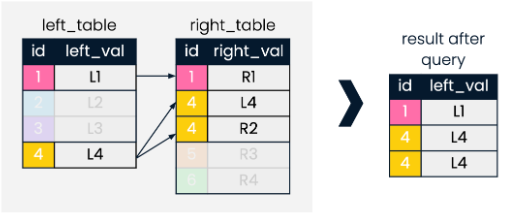
SELECT left_table.id, left_val 
FROM left_table, right_table
WHERE left_table.id = right_table.id  

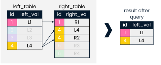
To drop the duplicates, we can use the distinct command:

SELECT DISTINCT left_table.id, left_val 
FROM left_table, right_table
WHERE left_table.id = right_table.id    

Continents with Monarchs

Suppose we want to find all continents with monarchs, along with the most recent country to gain independence in each continent.

First, we need a query to find the most recent independence year for each continent.

SELECT continent, MAX(independence_year) AS most_recent
FROM countries
GROUP BY continent;

Explanation:

• The query groups records by continent.
• It uses the MAX() function to find the most recent independence_year for each continent.
• The result provides the latest year of independence for each continent.

To filter this list for continents that have monarchs, we can include the subquery in the FROM clause.

SELECT DISTINCT monarchs.continent, sub.most_recent
FROM monarchs, (
    SELECT 
      continent, 
      MAX(independence_year) AS most_recent
    FROM countries
    GROUP BY continent
    ) AS sub
WHERE sub.continent = monarchs.continent
ORDER BY sub.continent;

Explanation:

• Subquery: The subquery in the FROM clause generates a temporary table with the most recent independence years, aliased as sub.
• Joining Tables: Both sub and monarchs are included in the FROM clause, separated by a comma, which allows us to reference both datasets.
• Filtering: The WHERE clause ensures we only include continents that have monarchs by matching sub.continent with monarchs.continent.
• Distinct Records: The DISTINCT keyword eliminates duplicate records in the result set.
• Ordering: The results are ordered by continent to improve readability.

Output:

Continent	most_recent
Asia	1991
Europe	1993

Common Table Expressions (CTEs)

CTEs create temporary, reusable result sets using the WITH keyword. They are ideal for large or complex datasets.

• Alternative to using JOINs.
• Creates a temporary table and gets executed only once.
• Improve readability by isolating query logic.
• Reduce redundant computations for better performance.

Example Use of CTEs:

• Aggregating word lengths in the English language using a CTE.
• Final query compares English word counts to movie script word counts.
• CTE improves speed by pre-aggregating data before joining.

When to Use:

• Use subqueries for simple calculations or dynamic filtering.
• Use CTEs for complex logic or large datasets needing optimization.

Climate Data for Southern Hemisphere Olympic Regions

Countries like Canada, Russia, and Mongolia have freezing temperatures year-round, while others experience winter cold for a few months, still supporting training for winter sports like skiing and bobsledding. Below are the sample datasets:

• athletes_recent.csv
• oclimate.csv

Examine temperature data for Olympic countries and focus on the southern hemisphere, which sees lower Winter Olympics participation.

• Write a CTE for the southern hemisphere.
• Find the average June temperature and precipitation.
• Join the data to see winter month temperatures for all regions.

Solution:

The CTE Calculates the average June temperature and precipitation for the specified regions. The JOIN Combines this data with athlete info for the winter season Finally, the GROUP and ORDER Groups results by region and averages, ordering by temperature.

WITH south_cte AS (
  SELECT region,
         ROUND(AVG(temp_06), 2) AS avg_winter_temp,
         ROUND(AVG(precip_06), 2) AS avg_winter_precip
  FROM oclimate
  WHERE region IN ('Africa', 'South America', 'Australia and Oceania')
  GROUP BY region
)

SELECT south.region, 
       south.avg_winter_temp, 
       south.avg_winter_precip,
       COUNT(DISTINCT ath.athlete_id)
FROM south_cte AS south
INNER JOIN athletes_recent ath
  ON south.region = ath.region
  AND ath.season = 'Winter'
GROUP BY south.region, south.avg_winter_temp, south.avg_winter_precip
ORDER BY south.avg_winter_temp;

Sample output:

Region	Avg Winter Temp (°C)	Avg Winter Precip (mm)	Count
South America	18.50	156.23	31
Australia and Oceania	19.87	137.92	76
Africa	23.99	73.98	5