Dates and Times
To run the code samples in this guide, check out the Jupyter notebook here: Using Pandas.
Loading Data
To learn more about datetime objects, please see Dates and Times in Python.
Pandas makes it easy to load and explore data from CSV files. We usually import it as pd and use read_csv() to load our data.
- Import Pandas with the alias
pd - Load CSV file using
pd.read_csv('filename.csv') - Store the result in a variable, e.g.,
my_var
In this example, we are using a bike CSV file, which contains ride data like start date, end date, start station, end station, bike number, and whether the rider is a member or casual user.
import pandas as pd

rides = pd.read_csv('capital_onebike.csv')
print(rides.head(3))
Expected output shows first 3 rows of the table with all columns and the index starting at 0.
            Start date             End date  Start station number  \
0  2017-10-01 15:23:25  2017-10-01 15:26:26                 31038
1  2017-10-01 15:42:57  2017-10-01 17:49:59                 31036
2  2017-10-02 06:37:10  2017-10-02 06:42:53                 31036

                   Start station  End station number  \
0           Glebe Rd & 11th St N               31036
1  George Mason Dr & Wilson Blvd               31036
2  George Mason Dr & Wilson Blvd               31037

                            End station Bike number Member type
0         George Mason Dr & Wilson Blvd      W20529      Member
1         George Mason Dr & Wilson Blvd      W20529      Casual
2  Ballston Metro / N Stuart & 9th St N      W20529      Member
Columns and Rows
We can access specific columns or rows easily.
- Get a column using
rides['Start date'] - Get a row using
rides.iloc[2] - Note that date columns are treated as strings by default
Working with strings for dates is limiting, so we usually convert them to datetime objects.
print(rides['Start date'])
print(rides.iloc[2])
Output:
0      2017-10-01 15:23:25
1      2017-10-01 15:42:57
2      2017-10-02 06:37:10
3      2017-10-02 08:56:45
4      2017-10-02 18:23:48
              ...
285    2017-12-29 14:32:55
286    2017-12-29 15:08:26
287    2017-12-29 20:33:34
288    2017-12-30 13:51:03
289    2017-12-30 15:09:03
Name: Start date, Length: 290, dtype: object
Start date                               2017-10-02 06:37:10
End date                                 2017-10-02 06:42:53
Start station number                                   31036
Start station                  George Mason Dr & Wilson Blvd
End station number                                     31037
End station             Ballston Metro / N Stuart & 9th St N
Bike number                                           W20529
Member type                                           Member
Name: 2, dtype: object
This lets us select and inspect data before doing any calculations.
Converting Columns to Datetime
Pandas can automatically convert columns to datetime when loading CSVs.
- Use
parse_datesargument inread_csv() - Pass a list of column names to convert, e.g.,
['Start date', 'End date'] - Pandas guesses the format; use
pd.to_datetime()if needed
rides = pd.read_csv('capital_onebike.csv',
                     parse_dates=['Start date', 'End date'])
print(type(rides.loc[2, 'Start date']))
Output:
<class 'pandas._libs.tslibs.timestamps.Timestamp'>
Now the Start date column is a Timestamp, and you can do all datetime operations on it (like .year, .month, .hour, arithmetic, etc.).
For example:
ride_start = rides.loc[2, 'Start date']
print(ride_start.year)
print(ride_start.month)
print(ride_start + pd.Timedelta(hours=2))
Output:
2017
10
2017-10-02 08:37:10
Calculating Duration
Once dates are datetime objects, we can calculate durations easily by subtracting the Start date column from the End date column. The result is a timedelta for each row.
ride_durations = rides['End date'] - rides['Start date']
rides['Duration'] = ride_durations.dt.total_seconds()

print(rides['Duration'].head())
This shows ride lengths in hours, minutes, and seconds.
0     181.0
1    7622.0
2     343.0
3    1278.0
4    1277.0
Name: Duration, dtype: float64
Summarizing Data
Pandas makes it easy to summarize data, including datetime columns. Make sure you are using Pandas version 0.23 or newer, because older versions may not support some methods.
- Use
.mean(),.median(),.sum()on numeric columns - Group by columns or time using
.groupby()or.resample() - Convert durations to seconds for easier calculations
Calculating Mean and Total
Numeric columns like Duration can be summarized directly.
rides['Duration'].mean()gives the average ride timerides['Duration'].sum()gives total ride time over a period
average_duration = rides['Duration'].mean()
total_duration = rides['Duration'].sum()

print(average_duration)
print(total_duration)
Output:
1178.9310344827586
341890.0
The mean shows typical ride length, and the sum shows how long bikes were out in total. You can also combine with Python operations, like dividing by total days to get percentages.
rides['Duration'] = rides['End date'] - rides['Start date']

# Total duration bikes were out
total_duration_seconds = rides['Duration'].sum().total_seconds()

# total days in the dataset converted to seconds
total_period_seconds = 91 * 24 * 60 * 60  # 91 days in seconds

# Fraction of time bikes were out
percent_out_of_dock = total_duration_seconds / total_period_seconds
print(percent_out_of_dock)
Output:
0.04348417785917786
Based on the output, we can see that bikes were out of the dock about 4.3% of the time.
Summarizing Non-Numeric Columns
For categorical data, Pandas has special methods:
- Use
.value_counts()to count occurrences of each value - Divide counts by total rows with
len(rides)to get percentages
member_counts = rides['Member type'].value_counts()
member_percent = member_counts / len(rides)

print(member_counts)
print(member_percent)
Output:
Member type
Member    236
Casual     54
Name: count, dtype: int64
Member type
Member    0.813793
Casual    0.186207
Name: count, dtype: float64
Here, we can see that 236 rides were from members and 54 were from casual riders, who bought a ride at the bike kiosk without a membership.
Member    236
Casual     54
Using value_counts() gives the number of rides per member type, and dividing by the total number of rides (len(rides)) gives percentages. The percentages make it easier to see how common each type of rider is.
The output shows that about 81% of rides were from members and 19% were from casual riders, which clearly highlights that most rides come from members.
Member    0.813793
Casual    0.186207
Grouping by Columns
You can use .groupby(column) to group rows and summarize each group separately. You can also apply aggregation methods like mean(), sum(), size(), or first() on each group.
rides['Duration seconds'] = rides['Duration'].dt.total_seconds()
grouped = rides.groupby('Member type')['Duration seconds'].mean()
print(grouped)
Output:
Member type
Casual    1994.666667
Member     992.279661
Name: Duration seconds, dtype: float64
This shows that casual rides are usually longer than member rides. Grouping lets you compare different categories easily.
Grouping by Time
Datetime columns can also be grouped by time using .resample().
.resample('M', on='Start date')groups rides by month- Aggregations like
mean()can be applied to each time period
monthly_avg = rides.resample('ME', on='Start date')['Duration seconds'].mean()
print(monthly_avg)
Output:
Start date
2017-10-31    1886.453704
2017-11-30     854.174757
2017-12-31     635.101266
Freq: ME, Name: Duration seconds, dtype: float64
This shows trends over time. For example, average ride durations may decrease from October to December.
Plotting Summaries
Pandas can plot grouped data quickly.
- Add
.plot()at the end of your summary to visualize results - ResamplING can be monthly(
M) or daily (D)
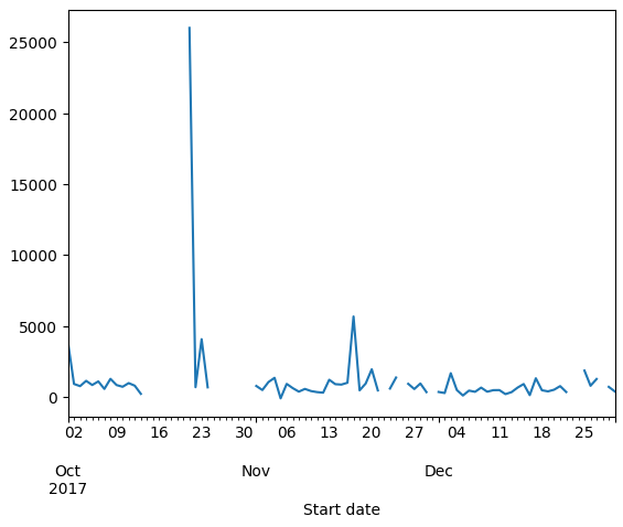
rides.resample('D', on='Start date')['Duration seconds'].mean().plot()
Plotting makes it easier to spot outliers, like a ride that lasted 25,000 seconds, which could indicate a bike repair.
Working with Timezones
Handling timezones is important to get accurate results with datetime data. Ride durations can appear negative if timezones are ignored, especially around Daylight Saving changes.
- Timezone-naive datetimes have no UTC offset
- dt.tz_localize() adds a timezone to a datetime column
We can use dt.tz_localize() to add a timezone to a datetime column and apply the correct UTC offset, which fixes errors caused by Daylight Saving.
# Localize the first three Start dates to America/New_York
rides['Start date'].head(3).dt.tz_localize('America/New_York')
Output:
0   2017-10-01 15:23:25-04:00
1   2017-10-01 15:42:57-04:00
2   2017-10-02 06:37:10-04:00
Name: Start date, dtype: datetime64[ns, America/New_York]
After localization, datetimes show a UTC offset and calculations become correct.
Handling Ambiguous Times
Sometimes a datetime falls during a Daylight Saving transition, causing an AmbiguousTimeError. You can resolve it by using the ambiguous argument in dt.tz_localize().
Setting ambiguous='NaT' marks the problematic rows as Not a Time, which Pandas ignores in calculations.
# Make timezone-aware in America/New_York
rides['Start date'] = rides['Start date'].dt.tz_localize('America/New_York', ambiguous='NaT')
rides['End date'] = rides['End date'].dt.tz_localize('America/New_York', ambiguous='NaT')

# Calculate durations in seconds
rides['Duration'] = (rides['End date'] - rides['Start date']).dt.total_seconds()

# Check minimum duration
print(rides['Duration'].min())
Output:
116.0
Rows that were ambiguous now have NaT for Start date or End date, so their Duration is also NaT. Pandas safely ignores these when performing aggregations.
To inspect the problematic rows:
rides[rides['Duration'].isna()]
Output:

Since we know that the row we want is at 129, we can use iloc to access it directly.
rides.iloc[129]
This returns the same output:
Start date                        NaT
End date                          NaT
Start station number            31615
Start station           6th & H St NE
End station number              31627
End station             3rd & M St NE
Bike number                    W20529
Member type                    Member
Duration                          NaN
Duration seconds              -3346.0
Name: 129, dtype: object
This shows all the details for that ride, including start and end stations, bike number, member type, and duration. Some values, like Start date and Duration, may be missing or invalid, which can happen in real datasets.
Other Datetime Operations
Pandas has many convenient datetime attributes and methods beyond basic Python:
dt.year,dt.month,dt.dayto access parts of the datetimedt.day_name()returns the day of the week- You can group and aggregate data by year, month, or day name
In this example, we use the .dt accessor to get parts of the datetime. The first line gets the year of each ride, and the second line gets the name of the weekday.
rides['Start date'].dt.year.head(3)
rides['Start date'].dt.day_name().head(3)
Output:
0    Sunday
1    Sunday
2    Monday
Name: Start date, dtype: object
Here, we can see that the first two rides started on a Sunday and the third ride started on a Monday.
Shifting Rows
Pandas allows shifting rows up or down with shift(). This is useful for comparing consecutive rides.
shift()moves rows up or down- Useful to align previous row data with current row
NaTfills the empty positions created by the shift
Example: Shifting rides one row forward
We can use shift(1) to move the Start date values down by one row. This is useful for comparing each ride to the previous ride.
rides['Start date'].shift(1).head(3)
Output:
0                         NaT
1   2017-10-01 15:23:25-04:00
2   2017-10-01 15:42:57-04:00
Name: Start date, dtype: datetime64[ns, America/New_York]
Here, we can see that the first row has no previous ride (NaT), the second row shows the first ride’s start time, and the third row shows the second ride’s start time. This helps calculate the time between rides.
Examples
How Many Joyrides?
“Joyrides” are rides that start and end at the same dock. We only have data for one bike, but it’s interesting to see how many there are and how long they last.
Use the median duration instead of the mean, since a few very long trips could skew the average.
rides['Duration'] = (rides['End date'] - rides['Start date']).dt.total_seconds()

# Create joyrides
joyrides = (rides['Start station'] == rides['End station'])
print("{} rides were joyrides".format(joyrides.sum()))

# Median of all rides
print("The median duration overall was {:.2f} seconds"\
      .format(rides['Duration'].median()))

# Median of joyrides
print("The median duration for joyrides was {:.2f} seconds"\
      .format(rides[joyrides]['Duration'].median()))
Output:
6 rides were joyrides
The median duration overall was 660.00 seconds
The median duration for joyrides was 2642.50 seconds
This shows that there were 6 joyrides, with a median duration of about 44 minutes, which is much longer than the overall median of 11 minutes. This suggests that joyrides tend to last longer than regular rides.
Members vs Casual Riders Over Time
Riders are either "Members," who pay yearly for unlimited bike access, or "Casual," who pay at the kiosk for single rides.
We want to see if members and casual riders decrease at the same rate from October to December, or if one group drops off faster.
We can use the Pandas method value_counts() to count how many rides come from members versus casual riders.
monthly_rides = rides.resample('ME', on='Start date')['Member type']

# Ratio of the .value_counts() over the total number of rides
print(monthly_rides.value_counts() / monthly_rides.size())
Output:
Start date  Member type
2017-10-31  Member         0.768519
            Casual         0.231481
2017-11-30  Member         0.825243
            Casual         0.174757
2017-12-31  Member         0.860759
            Casual         0.139241
dtype: float64
This shows that in October, about 77% of rides were from members and 23% from casual riders. By December, the percentage of member rides increased to about 86%, while casual rides dropped to about 14%. This indicates that casual riders decreased faster than members over the months.
Median Ride Duration by Member Type
We can see how ride lengths differ between members and casual riders over time. Using groupby('Member type').resample() lets us calculate statistics like the median ride duration for each month and membership type.
grouped = rides.groupby('Member type')\
               .resample('ME', on='Start date')

print(grouped['Duration'].median())
Output:
Member type  Start date
Casual       2017-10-31    1636.0
             2017-11-30    1159.5
             2017-12-31     850.0
Member       2017-10-31     671.0
             2017-11-30     655.0
             2017-12-31     387.5
Name: Duration, dtype: float64
This shows that casual riders had longer median rides than members in each month.
For example, in October, the median ride for casual riders was 1636 seconds (about 27 minutes), while for members it was 671 seconds (about 11 minutes). This pattern continues in November and December, with casual rides consistently being longer than member rides.
How Long Per Weekday?
We can find the median ride duration for each day of the week. The code adds a new column for the weekday of each ride, then groups rides by that weekday to calculate the median duration.
rides['Ride start weekday'] = rides['Start date'].dt.day_name()
print(rides.groupby('Ride start weekday')['Duration'].median())
Output:
Ride start weekday
Friday       724.5
Monday       810.5
Saturday     462.0
Sunday       917.0
Thursday     652.0
Tuesday      641.5
Wednesday    585.0
Name: Duration, dtype: float64
This shows the median ride duration for each day of the week. For example, Sunday rides last about 917 seconds (15 minutes) while Saturday rides last 462 seconds (8 minutes). This helps understand how ride patterns change by weekday.
Time Between Rides
We can also see how much time passes between rides by shifting the previous ride’s end date and subtracting it from the current ride’s start date.
# Shift index of end date up one, then subtract it from  start date
rides['Time since'] = rides['End date'].shift(1)
rides['Time since'] = rides['Start date'] - rides['Time since']

# Move from a timedelta to a number of seconds
rides['Time since'] = rides['Time since'].dt.total_seconds()

monthly = rides.resample('ME', on='Start date')
print(monthly['Time since'].mean() / (60*60))
Output:
Start date
2017-10-31 00:00:00-04:00    5.519242
2017-11-30 00:00:00-05:00    7.256474
2017-12-31 00:00:00-05:00    9.202380
Name: Time since, dtype: float64
This shows the average number of hours between rides each month. This gives insight into ride frequency and how busy the system is over time.