Functions

Updated Nov 20, 2022 ·

Overview

PromQL includes a variety of functions for performing calculations and transformations on time series data. These functions allow you to manipulate and query your metrics to gain deeper insights.

Math Functions

PromQL provides several mathematical functions to manipulate time series values. These functions allow you to apply standard mathematical operations such as rounding, absolute values, and more.

Consider the sample vector below:

$ node_cpu_seconds_total

node_cpu_seconds_total{cpu="0", mode="idle"}  4526.158
node_cpu_seconds_total{cpu="0", mode="user"}  2084.302
node_cpu_seconds_total{cpu="1", mode="idle"}  2535.042
node_cpu_seconds_total{cpu="1", mode="user"}  981.903
node_cpu_seconds_total{cpu="2", mode="idle"}  5026.302

Using the math functions:

• ceil function

  The ceil function rounds the values of a time series up to the nearest integer.

  Example:

  ceil(node_cpu_seconds_total)

  Output:

  node_cpu_seconds_total{cpu="0", mode="idle"}  4527
  node_cpu_seconds_total{cpu="0", mode="user"}  2085
  node_cpu_seconds_total{cpu="1", mode="idle"}  2536
  node_cpu_seconds_total{cpu="1", mode="user"}  982
  node_cpu_seconds_total{cpu="2", mode="idle"}  5027

• floor function

  The floor function rounds the values of a time series down to the nearest integer.

  Example:

  floor(node_cpu_seconds_total)

  Output:

  node_cpu_seconds_total{cpu="0", mode="idle"}  4526
  node_cpu_seconds_total{cpu="0", mode="user"}  2084
  node_cpu_seconds_total{cpu="1", mode="idle"}  2535
  node_cpu_seconds_total{cpu="1", mode="user"}  981
  node_cpu_seconds_total{cpu="2", mode="idle"}  5026

• abs function

  The abs function returns the absolute value of the time series, which makes all negative numbers positive.

  Example:

  abs(node_cpu_seconds_total - 5000)

  Output:

  node_cpu_seconds_total{cpu="0", mode="idle"}  526.158
  node_cpu_seconds_total{cpu="0", mode="user"}  -2915.698
  node_cpu_seconds_total{cpu="1", mode="idle"}  -2464.958
  node_cpu_seconds_total{cpu="1", mode="user"}  -4018.097
  node_cpu_seconds_total{cpu="2", mode="idle"}  26.302

Date and Time Functions

PromQL offers several functions to work with time-related data, helping you query and calculate metrics based on time.

time() 

Output:

time() 1671536400

To calculate how long the processes have been running:

time() - process_start_time_seconds

Output:

time() - process_start_time_seconds 200000

Other more granular functions are:

Function	Description
Minute()	Extracts the minute of the time.
Hour()	Extracts the hour of the time.
Day_of_the_week()	Returns the day of the week (0-6).
Day_of_the_month()	Returns the day of the month (1-31).
Days_in_month()	Returns the number of days in the month.
Month()	Returns the month (1-12).
Year()	Returns the year (e.g., 2024).

Changing Data Types

We can use vector functions to convert a scalar value into an instant vector.

scalar_to_vector(5) 

Output:

scalar_to_vector(5) 5

On the other hand, we can also convert an instant vector into a scalar function:

avg(node_cpu_seconds_total) 

Output:

avg(node_cpu_seconds_total) 1234.56

Sorting Functions

PromQL provides sorting functions that allow you to arrange your metrics in ascending or descending order. The example below sorts in ascending order.

$ sort(node_filesystem_avail_bytes)

node_filesystem_avail_bytes{device="sda1", fstype="ext4", instance="node1"}       1023
node_filesystem_avail_bytes{device="sda2", fstype="ext4", instance="node1"}       1587
node_filesystem_avail_bytes{device="sdb1", fstype="xfs", instance="node1"}        2003
node_filesystem_avail_bytes{device="sdb2", fstype="xfs", instance="node1"}        2459
node_filesystem_avail_bytes{device="sdc1", fstype="ext4", instance="node1"}       3067
node_filesystem_avail_bytes{device="sdc2", fstype="ext4", instance="node1"}       3672
node_filesystem_avail_bytes{device="sdd1", fstype="xfs", instance="node1"}        4321
node_filesystem_avail_bytes{device="sdd2", fstype="xfs", instance="node1"}        5184

To sort in descending order:

$ sort_desc(node_filesystem_avail_bytes) 

node_filesystem_avail_bytes{device="sdd2", fstype="xfs", instance="node1"}        5184
node_filesystem_avail_bytes{device="sdd1", fstype="xfs", instance="node1"}        4321
node_filesystem_avail_bytes{device="sdc2", fstype="ext4", instance="node1"}       3672
node_filesystem_avail_bytes{device="sdc1", fstype="ext4", instance="node1"}       3067
node_filesystem_avail_bytes{device="sdb2", fstype="xfs", instance="node1"}        2459
node_filesystem_avail_bytes{device="sdb1", fstype="xfs", instance="node1"}        2003
node_filesystem_avail_bytes{device="sda2", fstype="ext4", instance="node1"}       1587
node_filesystem_avail_bytes{device="sda1", fstype="ext4", instance="node1"}       1023

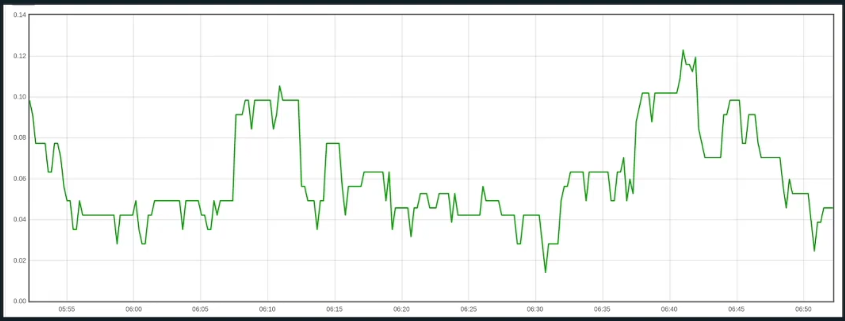
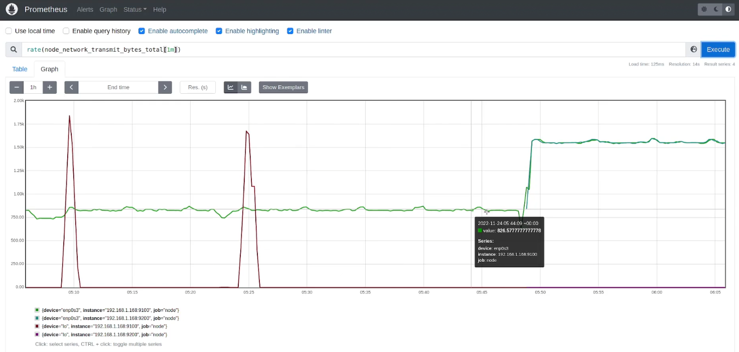
Rate

We can use rate to plot a metric and observe the rate at which it increases over time. To achieve this, we use the rate() and irate() functions, which calculate the per-second average rate of change of a time series over a specified period.

• rate()

  • Computes the average rate of change over a time interval.
  • Looks at first and last data points within a range.
  • Effectively an average rate over the range.
  • Best used for counters and alerting rules.

• irate():

  • Computes the instantaneous rate of change.
  • Based on the most recent two data points.
  • Looks at the last two data points within a range.
  • Provides a better representation of the instant rate,
  • Used for graphing volatile, fast-moving counters.

These functions are useful when monitoring time series metrics, such as counters, to understand how fast the values are changing.

A few important reminders when using rate() and irate() in PromQL:

• Ensure there are at least 4 samples within the given time range for accurate calculations.
• If you have a 15-second scrape interval, a 60-second window will provide 4 samples.
• When combining with an aggregation operator:
  • Use rate() first to detect counter resets.
  • After applying rate(), you can aggregate the results with functions like sum().