Subqueries and Histograms
Subqueries
Subqueries allow you to perform calculations over a range of data within another query. This makes them useful for detailed analysis. They enable combining multiple time ranges and resolutions in a single query. Subqueries follow this format:
<instant_query> [<range>:<resolution>] [offset <duration>]
For example, the following query analyzes a 1-minute sample range, a 5-minute query range (data from the last 5 minutes), and uses a 30-second step size for subquery resolution:
rate(http_requests_total[1m]) [5m:30s]
This returns a range vector:
0.9945645655554557 @1664226130
1.0234542343346789 @1664226160
0.9865432345435432 @1664226190
1.0456789876543210 @1664226220
1.0123456789123456 @1664226250
0.9754323456789123 @1664226280
The output can then be passed to max_over_time to calculate the maximum rate of requests over the last 5 minutes, with 30-second intervals and a 1-minute sample range:
max_over_time(rate(http_requests_total[1m]) [5m:30s])
Output:
1.0456789876543210 @1664226220
Histograms
Histograms in PromQL are used to observe and analyze distributions of sample values over a range. They provide insights into metrics by dividing them into cumulative buckets.
In the example below, we have three sub-metrics within a histogram metric:
request_latency_seconds_count: Represents the total number of samples.request_latency_seconds_sum: Represents the sum of all the samples.request_latency_seconds_bucket: Contains all the samples for each bucket value.
Checking the sixth line in the image, we see that there are 50 requests with latencies less than 0.05 seconds.
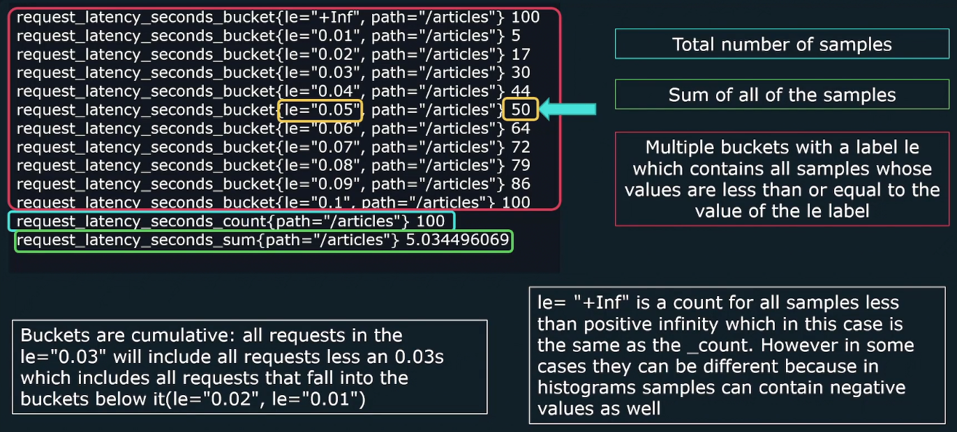
Note that buckets are cumulative, meaning each bucket includes all requests with values less than or equal to the le label. For example, le="0.05" includes all requests falling below 0.05 seconds, as well as those in smaller buckets like le="0.04" and le="0.03".
For the requests_latency_seconds_count metric, we don't care about the number since it's a counter; it will always go up. Instead, we want to know the rate at which it increases.
Here are some more sample queries:
-
The query below will return an instant vector.
rate(requests_latency_seconds_count[1m]) -
To get a range vector, we can use:
rate(requests_latency_seconds_count[1m]) [5m:30s]
-
We can also get the rate of requests for each bucket by running:
rate(requests_latency_seconds_bucket[1m]) [5m:30s]
-
To get the total sum of latency across all requests:
requests_latency_seconds_sum -
To get the rate of increase of the sum of latency across all requests:
rate(requests_latency_seconds_sum[1m]) -
To calculate the average latency of a request over the past 5m
rate(requests_latency_seconds_sum[5m]) rate(requests_latency_seconds_count[5m]) -
To calculate percentage of requests that fal into a specific bucket
rate(request_latency_seconds_bucket(path="/articles", le="0.06">[1m]) / ignoring(le) rate(request_latency_seconds_countfpath="/articles")[1m]) -
To calculate the number of observations between two buckets
request_latency_seconds_bucket(path="/articles", le="0.06") - request_latency_seconds_bucket(path="/articles", le="0.03")
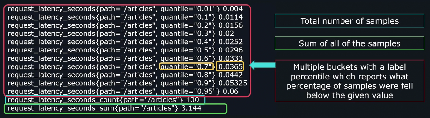
Quantiles
Quantiles help determine the value below which a certain percentage of observations fall, providing insights into data distribution. They are commonly used to assess performance metrics like latency at specific thresholds.
- Quantiles represent specific percentiles.
- For example, the 90% quantile indicates the value below which 90% of the data points fall.
To easily compute the quantile, histogram has a function called histogram_quantile().

Measuring SLO
Histogram quantiles are useful for determining whether a specific Service Level Objective (SLO) is being met and can trigger alerts if the SLO is exceeded.
-
Example: The SLO states that 90% of requests must not exceed 0.5 seconds.
-
Using the histogram function:
histogram_quantile(0.90, rate(request_latency_seconds_bucket[5m])) -
If the output is greater than 0.5 seconds, the SLO is not met.
Using Linear Interpolation
Histogram quantiles use linear interpolation to estimate values, which can lead to inaccuracy when measuring SLOs. To ensure accuracy, make sure there is a bucket at the specific SLO value.
Example: For an SLO requiring 90% of requests to have latency below 0.5 seconds:
- Ensure one bucket is set to 0.5.
- Allows precise checking of whether 90% of requests meet the SLO.
Note that even with a bucket at the SLO value, it won’t tell us exactly how much we missed the SLO or how close we were. Proper bucket configuration is crucial for better accuracy.
- Example bucket setup: 0.1, 0.2, and 0.5
- If the quantile reports 0.4, the actual value lies between 0.2 and 0.5.
- For more precision, add additional buckets between 0.2 and 0.5.
Too Many Buckets
Each histogram creates separate time series, so having too many buckets can lead to:
- High cardinality
- Increased RAM usage
- Higher disk space consumption
- Slower database insert performance
This means excessive buckets can strain system resources, reduce query efficiency, and impact overall performance.
Summary Metrics
Summary metrics provide a way to measure data distribution, similar to histograms, but with predefined quantiles for faster calculations.
Just like histograms, summary metrics have three sub-metrics:
_count: Total number of samples._sum: Sum of all sample values._bucket: Contains samples grouped by bucket values.
To get a specific quantile, use:
request_latency_seconds{quantile="0.5"}
Histograms vs. Summary
-
Histograms
- Flexible bucket sizes.
- Lighter load on client libraries.
- Any quantile can be calculated.
- Prometheus calculates quantiles server-side.
-
Summary
- Quantiles must be predefined.
- Heavier load on client libraries.
- Only predefined quantiles are available.
- Minimal server-side processing.